Magnetic resonance (MR) imaging based measurements of cartilage morphology are being used increasingly as a quantitative end point of disease status and a marker of disease progression in osteoarthritis.^1–3 This technique can be employed either to measure structural changes in the joint longitudinally^3–5 or to grade cartilage status in cross sectional studies,^2,6,7 for instance at the onset of symptomatic osteoarthritis. Accurate retrospective estimates of cartilage loss are also important when determining the appropriate time point and type of treatment for patients with osteoarthritis, in carrying out cross sectional epidemiological studies, or when selecting specific patient groups for longitudinal trials. However, one problem with such retrospective estimates is the relatively large intersubject variability of normal (healthy) cartilage morphology.^6–9 Also there is a lack of strong correlation with anthropometric factors such as age, body height and weight, and muscle cross sectional area.^7,8,10 These two factors render the retrospective estimate of the “original” cartilage volume (before the onset of disease) and of the amount of cartilage loss (original cartilage volume minus currently measured cartilage volume) a diagnostic and scientific challenge.⁷

It has been shown previously that differences in cartilage volume, thickness, and surfaces area in healthy contralateral knees are relatively small.¹¹ Thus in a case of unilateral osteoarthritis it may be feasible to estimate the original cartilage morphology from the contralateral (unaffected) joint. However, strictly unilateral knee osteoarthritis is rare, and early morphological changes in the contralateral knee are difficult to rule out with certainty.

Another possible approach to resolve this challenge is to measure a cartilage plate in another joint which is less often affected by primary osteoarthritis, such as the ankle.^12–14 If a strong correlation of cartilage morphology between the knee and ankle can be established in healthy subjects, and if osteoarthritic changes in the ankle are not associated with osteoarthritic changes in the knee, it may be possible (a) to estimate the original cartilage volume (before osteoarthritis) in the knee by measuring cartilage volume in a healthy ankle and applying a scaling factor based on an established regression equation (fig 1); and (b) to estimate tissue loss by subtracting the current measured cartilage volume in the knee (with osteoarthritis) from the estimated original cartilage volume (before osteoarthritis), as described in (a).

• Download figure
• Open in new tab
• Download powerpoint

Figure 1

 Scattergram showing the rationale for the study. If the hypothesis is correct that there is a strong linear relation between knee joint cartilage volume in the knee and ankle surfaces (for example, medial tibia and distal tibia) in healthy volunteers (empty circles), this relation can be exploited to estimate retrospectively the amount of tissue loss in the knee surface in a cross sectional study. In the 29 healthy volunteers examined in this study, the cartilage volume of the medial tibia (knee joint) varied from 1.1 to 3.2 ml (mean 2.3 ml), and that of the distal tibia (ankle joint) from 0.6 to 1.7 ml (mean 1.1 ml). The graph also shows the hypothetical measurement in a patient (filled circle). Assuming a strong linear relation in healthy volunteers (empty circles), one could accurately estimate the cartilage tissue loss in the medial tibia of the hypothetical patient to amount to 1.2 ml (50% cartilage loss), although the measurement at the knee of this patients falls within the normal range.

As mentioned previously, the potential for these estimates to be useful is dependent on a strong correlation between knee and ankle cartilage volume in health. The stronger the correlation coefficient and the narrower the standard error of the estimate between knee and ankle cartilage morphology, the more precise the estimate. Our primary objective in this study was thus to examine the association between cartilage morphology in the healthy knee and ankle (fig 1). The ankle (and subtalar) joints were selected for the following reasons: first, they show much lower susceptibility to and severity of osteoarthritis than the knee^12–14; second, they represent lower limb joints that encounter similar loading profiles to the knee; third, they can be imaged using a circumferential coil with high signal homogeneity and a high contrast to noise ratio; and fourth, they allow for quantitative measurements of cartilage indices with satisfactory reproducibility (precision) in vivo.¹⁵

The second objective of this study was to investigate sex differences in quantitative cartilage indices at the ankle and knee. Although women over the age of 50 show a higher incidence of knee osteoarthritis than men of the same age,¹⁶ osteoarthritis of the ankle is somewhat more frequent in men.¹⁴ It has been speculated that differences in accrual of knee cartilage during adolescence may be responsible for sex differences in susceptibility to knee osteoarthritis later in life.^17,18 It has also been reported that, in the knee, sex differences in joint surfaces area are larger than those of cartilage thickness.¹⁹ We therefore tested the hypothesis that sex differences in knee cartilage morphology are larger than those in the ankle and subtalar joints, potentially explaining the higher incidence of knee osteoarthritis in elderly women.

METHODS

Study subjects

We examined 29 healthy volunteers with no history of knee or ankle pain, trauma, surgery, or ligament or meniscal lesions. Fourteen of the subjects were women (mean (SD) age, 25.0 (4.2) years), and 15 were men (age 24.7 (2.1) years). The men were significantly taller (180 (4.8) v 167 (7.8) cm; p<0.001) and heavier (72.6 (7.1) v 59.0 (6.4) kg; p<0.001) than the women, but the mean body mass index was similar (22.4 (2.2) v 21.4 (3.8) kg/m²). Informed written consent was obtained from each subject, and the consent form and study protocol were ratified by the local ethic committee.

MR image acquisition and analysis

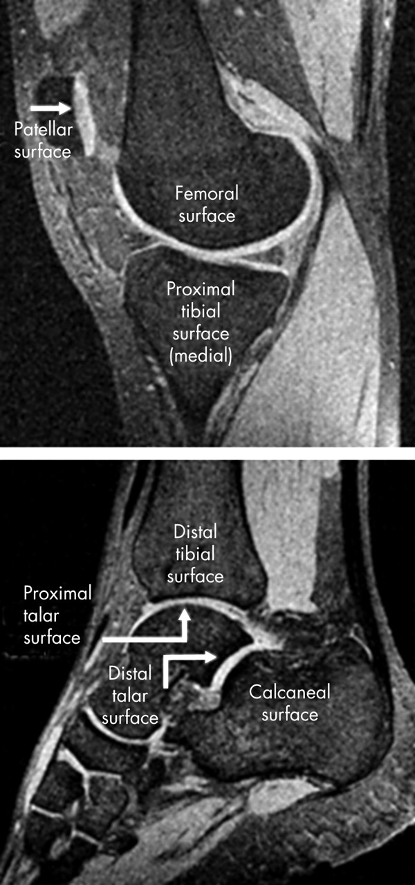
Imaging was carried out with a 1.5 T MR scanner (Magnetom Vision, Siemens, Erlangen, Germany) and a circularly polarised transmit–receive extremity coil. A sagittal T1 weighted 3D FLASH (fast low angle shot) MR sequence with selective water excitation (RF amplitude ratios 1–2–1; time of repetition (TR) = 18 ms, time of echo (TE) = 9 ms; flip angle (FA) = 25, band width = 105 Hz/pixel) was used for the hind foot¹⁵ (resolution 1×0.25×0.25 mm; field of view (FOV) = 12 cm; matrix = 512×512; number of excitations (NEX) = 2; acquisition time = 19 minutes) and a similar sequence (TR = 17.2 ms, TE = 6.6 ms; FA = 25) for the knee joint²⁰ (resolution 1.5×0.31×0.31 mm; FOV = 16 cm, matrix = 512×512; NEX = 1, acquisition time = 9 minutes) (fig 2). These MR sequences have previously been shown to yield accurate (valid) results for quantitative indices of cartilage morphology in the knee joints of healthy volunteers,²⁰ in patients with severe osteoarthritis,^2,21 and in joints with thin cartilage.^22,23 In 16 volunteers (eight women, eight men) additional axial spin echo images at the thigh (at 50% of the distance between the greater trochanter and knee joint space) and at the maximum circumference of the calf) were acquired to determine muscle cross sectional areas at these locations.¹¹

• Download figure
• Open in new tab
• Download powerpoint

Figure 2

 Sagittal magnetic resonance images of the knee and ankle, acquired with a high resolution FLASH (fast low angle shot) wider excitation sequence. The figure also displays the surfaces that have been analysed in the current study.

An Octane Duo work station (Silicon Graphics Inc, Mountain View, California, USA) was used for digital image analysis. A semiautomated B-spline Snake algorithm was employed for segmentation of the distal tibial and proximal talar cartilage plate (ankle joint), the distal talar and calcaneal cartilage plate (subtalar joint), and the patellar, femoral, and proximal tibial cartilage plates (knee joint).²⁴ The cartilage volume of each plate was determined by numerical integration of the attributed voxels,²⁵ and the size of the joint surface area (JSA) and bone–cartilage interface (BCI) with a validated triangulation algorithm.²⁶ The mean and maximum cartilage thickness were determined, independent of the original section orientation, using three dimensional Euclidean distance transformation.²⁷ The total cartilage volume and surface areas in the ankle, subtalar, and knee joints were obtained by summing the surfaces within each joint. The mean cartilage thickness was computed by weighting the mean thicknesses of the relevant joint surfaces with their relative proportion of the total joint surface area.^8,15 The in vivo reproducibility of the imaging protocols and analysis steps have been reported previously.^15,28 Test–retest precision errors (with joint repositioning) ranged from 2.0% to 3.6% (CV%) in the knee, and from 2.1% to 8.1% in the ankle and subtalar joint. The muscle cross sectional areas (MCSAs) of the thigh (quadriceps, adductors, and flexors) and calf (mainly triceps surae) were determined with the same segmentation tool,²⁴ and subcutaneous fat, muscle septs with adipose tissue, and bones were eliminated from the analysis. The area was again determined by numerical integration of segmented voxels, and the precision for these measurements has been reported previously.¹⁰

Statistical analysis

The correlation between the ankle, subtalar, and knee joint surfaces, and the muscle cross sectional areas of the thigh and calf were determined by linear regression analysis (Pearson correlation coefficient and standard error of the estimate). Average correlation coefficients within the knee joint surfaces, within the hind foot cartilage plates, and between the knee and hind foot plates were determined by computing the means of correlation coefficients. Coefficients were compared in order to identify possible significant differences, using the Fisher z test. Sex differences were tested for statistical significance using an unpaired t test.

RESULTS

The cartilage volumes and joint surface areas of the knee showed only moderate correlations with those of the ankle and subtalar joint (r = 0.33 to 0.81; table 1). The correlation of mean cartilage thickness between the knee and ankle was weaker still (r = −0.05 to 0.53; table 1). Correlation coefficients between cartilage volumes of the knee and body height ranged from r = 0.54 (patella) to r = 0.79 (femur), and those for the ankle from r = 0.44 (calcaneus) to r = 0.51 (proximal talus). Correlation coefficients between cartilage thickness and body height were again lower and ranged from r = 0.05 (patella) to r = 0.64 (femur) in the knee, and from r = 0.17 (distal tibia) to r = 0.31 (distal talus) in the ankle.

The correlation of morphological indices among joint cartilage plates of the same joint (for example, within the knee) was stronger than that between cartilage plates of different joints (between knee and ankle) (table 2). The associations between the ankle and subtalar joint plates tended to be stronger than those between the ankle and knee joint and between and subtalar and knee joint, respectively. The correlation was generally stronger for joint surface areas (and cartilage volumes) than for cartilage thickness (table 1). The associations of cartilage volume, cartilage thickness, and surface area between the (total) knee, ankle, and subtalar joint are shown in fig 3. The standard error of the estimate (SEE)—that is, the standard error when attempting to estimate values for the dependent variable (for example, medial tibia) from the independent variable (such as ankle cartilage) in the regression—was 0.43 ml (19%) for the distal tibial surface (ankle joint) v medial tibial plateau (knee). The SEE was 0.40 ml (18%) when using the proximal talar surface (ankle joint), 0.41 ml (18%) when using the distal talar surface (subtalar joint), and 0.43 ml (19%) when using the calcaneal surface (subtalar joint) to estimate values in the medial tibial plateau of the knee. These standard errors were relatively large compared with the standard deviation/coefficient of variation (CV%) of the cartilage volume in the medial tibia of healthy women (0.37 ml/19%) and healthy men (0.44 ml/16%), respectively.

• Download figure
• Open in new tab
• Download powerpoint

Figure 3

 Bivariate scattergrams showing the correlation of cartilage volume in the knee, ankle, and subtalar joint. Women and men are identified in the graphs. Surface, joint surface area; thickness, mean cartilage thickness; volume, cartilage volume.

The knee joint cartilage plates tended to display a slightly stronger correlation with MCSA of the thigh than with MCSA of the calf (table 3). However, the cartilage plates of the hind foot did not consistently show a stronger correlation with MCSA of the calf than with MCSA of the thigh (table 3).

Sex differences in cartilage morphology were greater for the joint surface areas (range, −17.5% to −23.5%) than for the cartilage thickness (range, +4.1% to −19.5%). Sex differences ranged from −15.1% to −31.8% for cartilage volumes of the knee, ankle, and subtalar joint surfaces, and did not show any obvious differences between joints (tables 4 and 5).

DISCUSSION

Our study is the first to provide a comprehensive analysis of the correlation of cartilage morphology between two different joints in the human body. We have specifically tested the hypotheses that cartilage loss in gonarthritis can be estimated retrospectively by quantitative magnetic resonance imaging of the ankle and knee, and that sex differences in cartilage morphology are greater in the knee than in the ankle, which may explain the higher prevalence of knee osteoarthritis in elderly women. State of the art MR imaging and digital analysis technology were used to investigate these relations in vivo in young, healthy subjects without signs of osteoarthritis. The MR sequence and analysis tools have been validated previously and tested for reproducibility in vivo.^{2,15,20,28,29} Precision errors are substantially less than the intersubject variability reported for healthy volunteers in both the knee and the hind foot; therefore the results of this study should not be critically affected by measurement errors.

A strong correlation between human knee and ankle cartilage morphology could not be confirmed by our study, although all subjects were healthy and none had any signs of joint disease. The subjects were carefully selected for young age and lack of any history of ankle or knee pathology (pain, trauma, or surgery). Moreover, to ensure that the subjects showed no signs of osteoarthritis, the MR images were rated by an experienced radiologist (CG) and an experienced orthopaedic surgeon (HG). The low correlation between cartilage morphology in the knee and ankle cannot thus be explained by the detection of incipient osteoarthritis in either the knee or ankle.

The correlation coefficients between cartilage volumes in the knee and ankle cartilage plates were not higher than those between cartilage volumes and body height, a variable that is clearly more easily measured. A recent paper has shown that, given the correlation with body height is only moderate, normalisation of knee cartilage volume to height does not improve the discrimination between healthy subjects and patients with knee osteoarthritis. However, normalisation to the original (cartilaginous + eroded) joint surface area (as measured from MR image data by digital image analysis) can substantially increase t and z scores for osteoarthritis patients.⁷ Not only did we find that the correlation coefficients between knee and ankle cartilage morphology in healthy subjects were moderate and not significantly greater than the correclation with body height, but in practice it would also be difficult to rule out convincingly the possibility that no quantitative change had occurred in ankle cartilage morphology.

The standard error of the estimate of the regression between the hind foot and knee joint surfaces and the standard deviation of knee joint cartilage volume among healthy men and women were in the same range. The correlation was thus not strong enough and the standard error of the estimate not sufficiently narrow to provide more precise estimates of cartilage loss in knee osteoarthritis beyond guesses based on the normal variability of cartilage morphology in reference subjects. The correlation coefficients between different joints for joint surface area and cartilage volume were somewhat higher than for cartilage thickness, probably because bone size is less variable throughout the body and (metaphyseal) bone size is the main determinant of cartilage surface area (and to a lesser degree also of cartilage volume).

One potential explanation for the heterogeneity of cartilage thickness between different joints is a concomitant heterogeneity between relevant muscle forces acting across the joints. We have shown previously that MCSAs of the thigh are significant predictors of knee joint cartilage morphology and provide additional information independent of body size and weight.¹⁰ For this reason we tested the hypotheses that there is a stronger correlation between knee joint cartilage thickness and thigh MCSA and between ankle and subtalar joint cartilage thickness and calf MCSA than the converse relations. This would imply that the heterogeneity in regional muscle forces is responsible for the heterogeneity in cartilage morphology between different joints. This hypothesis was, however, falsified. It thus remains unclear which factors cause one joint surface to have a large and another a relatively small cartilage thickness within an individual.

Previous ex vivo studies have revealed fundamental biochemical and biomechanical differences between ankle and knee cartilage.^30–33 There are claims that these differences may also be responsible for the greater prevalence of cartilage lesions (osteoarthritis) in the knee than in the ankle.^32–34 We have previously observed that women have substantially smaller joint surface areas than men¹⁹; smaller joint surfaces potentially predispose women to larger mechanical stress on their knee joint surfaces. This, in turn, may lead to earlier and more severe damage to the cartilage and joint. Because women over the age of 50 have a higher prevalence of osteoarthritis in the knee, but men have a higher prevalence of osteoarthritis in the ankle, we tested the hypothesis that sex differences in ankle cartilage morphology are greater in the knee than in the hind foot. However, our findings show that the sex differences in the knee, ankle, and subtalar joints are similar. Sex differences in susceptibility to osteoarthritis between knee and ankle are therefore not readily explained by differences in joint surface areas. It has been suggested that hormonal factors may be associated with osteoarthritis in postmenopausal women. However, it is currently unclear whether women with hormone replacement therapy are less often affected by osteoarthritis, and how and why this mechanism should preferentially affect the knee.^35,36

Conclusions

We find that there is only a weak to moderate correlation of cartilage morphology between joint surfaces of the knee and the hind foot. This weak correlation makes it impractical to estimate knee joint cartilage loss retrospectively in a cross sectional study by measuring ankle cartilage and applying a scaling factor from an established regression equation. The heterogeneity of cartilage morphology between joints is not explained by differences in the local loading environment as there is no greater correlation with the relevant muscles (thigh versus calf). Sex differences were found to be of similar magnitude in the knee, ankle, and subtalar joint. The existing data do not support the hypotheses that sex differences in osteoarthritis incidence between the knee and ankle can be explained by differences in joint or cartilage morphology. Given the weak correlation between knee and ankle cartilage morphology, retrospective estimates of cartilage loss in cross sectional study designs must continue to rely on comparisons with samples of sex matched young subjects or age matched healthy volunteers, preferably with normalisation of cartilage volume to the “original” (cartilaginous + eroded) bone cartilage interface area.⁷