


Abstract
Marginal structural models (MSMs) are being used more frequently to obtain causal effect estimates in observational studies. Although the principal estimator of MSM coefficients has been the inverse probability of treatment weight (IPTW) estimator, there are few published examples that illustrate how to apply IPTW or discuss the impact of model selection on effect estimates. The authors applied IPTW estimation of an MSM to observational data from the Fresno Asthmatic Children's Environment Study (2000–2002) to evaluate the effect of asthma rescue medication use on pulmonary function and compared their results with those obtained through traditional regression methods. Akaike's Information Criterion and cross-validation methods were used to fit the MSM. In this paper, the influence of model selection and evaluation of key assumptions such as the experimental treatment assignment assumption are discussed in detail. Traditional analyses suggested that medication use was not associated with an improvement in pulmonary function—a finding that is counterintuitive and probably due to confounding by symptoms and asthma severity. The final MSM estimated that medication use was causally related to a 7% improvement in pulmonary function. The authors present examples that should encourage investigators who use IPTW estimation to undertake and discuss the impact of model-fitting procedures to justify the choice of the final weights.
Marginal structural models (MSMs) are being used more frequently to obtain causal effect estimates in observational studies (1–3), where causal effects are typically defined by a comparison of how a population mean outcome changes when the population exposure of interest changes. These models are appealing, because the coefficients are directly interpretable causally and they provide unbiased marginal estimates even in the presence of time-dependent confounding. Inverse probability of treatment weight (IPTW), G-computation, and double robust estimation methods are techniques used for causal modeling (4–6). To date, the principal estimator of MSM coefficients has been IPTW estimation, because of its relative ease of implementation. However, there are few simple examples that illustrate how to apply IPTW to obtain estimates of unconfounded causal associations between exposures and outcomes. Moreover, there has been little discussion of the importance of model-fitting of IPTW estimators of MSM coefficients and its influence on the validity of the results, and few studies have fully addressed a critical assumption, the experimental treatment assignment (ETA) assumption.
In this paper, we provide a step-by-step illustration of the conceptualization and implementation of IPTW estimation of an MSM to adjust for confounding and to obtain marginal causal effect estimates. We begin with an example of traditional association models and demonstrate problems related to confounding and interpretation. We then discuss steps necessary to estimate coefficients defined by MSMs. We examine the sensitivity of the findings to decisions about model selection and discuss the treatment of extreme values. Finally, we propose steps to provide a better understanding of one model-fitting process that can be used in the context of IPTW estimation and the interpretation of the results.
BACKGROUND
MSMs are based on the concept of counterfactual variables. Counterfactuals are sets of random variables that represent all of a study subject's possible outcomes, including the observed outcome and those outcomes that would occur if, contrary to fact, the subject were exposed to each possible exposure history (5). In the context of MSMs, exposures can be assigned at random or manipulated, and they are referred to as “treatments” in the relevant literature, although epidemiologists may use the term “exposure” more often. In an ideal experiment for the investigation of a causal effect, each subject receives every exposure (including no exposure), and the outcome under each exposure is observed. Such an experiment would permit direct estimation of the causal effect of the exposure of interest. In contrast, in observational studies, at any given time, only one exposure and the corresponding outcome are typically observed for each subject. This can be considered a missing-data problem, because not all possible exposure/outcome combinations are available.
APPLICATION
In observational studies, factors that influence the exposure assignment may also influence the outcome and, therefore, may confound the association of interest. A useful example occurs in observational studies of the effect of use of asthma rescue medication on pulmonary function measures. Asthma rescue medication provides a relatively short-acting but rapid improvement in lung function measures such as peak expiratory flow rate (PEFR). Medication use (exposure) is not randomized and is likely to be strongly related to the occurrence of prior asthma symptoms that also can be markers of asthma severity and thus influence PEFR. Therefore, because we are interested in the marginal (i.e., unconditional) causal effect of medication use on PEFR, confounding by prior symptoms must be considered. Although this is seldom stated, traditional methods of analysis estimate adjusted effects, but often the coefficient defined by association models cannot be interpreted causally. In a standard association model for the effect of medication use on PEFR that adjusts for prior symptoms, the implicit assumption that symptoms are held constant in the model would be violated, since a change in medication use would probably be accompanied by a change in symptoms. Therefore, coefficients in an association model would not be interpretable as the marginal causal effect of medication use on PEFR. The following examples demonstrate how failure to properly consider prior symptom status results in estimates that are contrary to the known pharmacologic effects of rescue medication use on PEFR. We demonstrate that MSMs lead to a less biased estimate of the causal effect.
Data were obtained from the Fresno Asthmatic Children's Environment Study, which examines the effect of air pollution on asthmatic children. The study was approved by the Committee for the Protection of Human Subjects of the University of California, Berkeley. Over several 2-week periods, children aged 6–11 years used a portable spirometer to obtain twice-daily readings of pulmonary function and completed questions related to symptoms and use of asthma rescue medications. This analysis includes 4,093 child-days of observation pertaining to 186 children. The principal outcome measure (Y) is defined as the mean of up to three acceptable PEFR values obtained during the morning testing session. The primary exposure (treatment) variable is the use of asthma rescue medications (A) in the hour prior to pulmonary function testing. The confounding variable of interest is reported symptoms (cough or wheeze (W)) experienced from the time the child went to bed until waking (i.e., symptoms that occurred prior to taking the PEFR measurement) (figure 1). The following notation defines the counterfactuals of interest: Ya, outcome Y measured under exposure value a, such that Y1= PEFR with treatment and Y0 = PEFR without treatment. The causal effect of interest can be defined as the difference in the mean pulmonary function levels of children who did and did not use rescue medication, in the situation where medication use is unconfounded and patients are fully compliant with the medication assignment (treated/untreated). A model for E(Y|A) cannot reveal a marginal causal effect, because the counterfactual PEFRs are not independent of A. However, an MSM can define such a causal effect. In the absence of such randomized data, we will discuss the estimation of MSMs to evaluate a causal effect based on observational data.
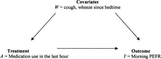
Theoretical association between symptoms, use of asthma rescue medication, and peak expiratory flow rate (PEFR).
The marginal causal effect at the individual level, Y1 − Y0, is inherently a counterfactual, since, at any given time for a child, we observe only the outcome under either the treated state (Y1) or the untreated state (Y0) but not under both states. Our goal then is to model, at the population level, the average marginal causal effect, which can be written as β1 = E(Y1 − Y0) = E(Y1) − E(Y0), where E(Y1) and E(Y0) are the population mean PEFRs when all children in the population did and did not take rescue medication, respectively. Thus, β1 is the average marginal causal effect of A (use of rescue medication) on Y (PEFR). In contrast, the causal effect, conditional on prior symptoms (W), can be defined by β1(W) = E(Y1 − Y0)|W) = E(Y1|W) − E(Y0|W), that is, the causal effect of A on Ya, conditional on W (prior symptoms). In practice, E(Y|A = 1, W = 1) represents the average PEFR among children with symptoms who used medication, whereas E(Y1|W = 1) represents the average PEFR among the children who had prior symptoms had those children also taken rescue medication—thus, for some, contrary to fact. These conditional expected values are equal only if medication use, A, is independent of the set of all counterfactuals (Ya) given W (prior symptoms). Under this independence condition, E(Y|A,W) = β0 + β1A + β2W is a model wherein β1 can be interpreted as the adjusted (pooled) causal effect, that is, the causal effect of A on Y per stratum of W.
The observed mean PEFR for the children who reported symptoms in the morning was significantly lower than that for the nonsymptomatic children, and prevalence of medication use was highly related to symptoms (table 1). Medication use should improve pulmonary function; however, children who took medication in the previous hour also had significantly lower mean PEFRs than unmedicated children (mean PEFR = 3.3 liters/second vs. 3.6 liters/second (95 percent confidence interval for difference: 0.17, 0.45)). This counterintuitive finding is probably due to confounding by symptoms (i.e., the reason the child took medication) rather than any negative medication effect. Children who took rescue medication may also have had more severe asthma, and therefore their mean PEFR may have remained lower despite medication use.
Peak expiratory flow rate and medication use by symptom category among participants in the Fresno Asthmatic Children's Environment Study, Fresno, California, November 2000–November 2002
Symptom category | Child-days | Probability of medication use | PEFR* | No medication use | Medication use | ||||||
|---|---|---|---|---|---|---|---|---|---|---|---|
| Mean | SE* | Mean PEFR | SE | Mean PEFR | SE | ||||||
| No cough and no wheeze | 2,913 | 0.02 | 3.7 | 0.02 | 3.7 | 0.02 | 3.4 | 0.15 | |||
| Either cough or wheeze | 703 | 0.10 | 3.4 | 0.04 | 3.5 | 0.05 | 3.2 | 0.12 | |||
| Both cough and wheeze | 477 | 0.43 | 3.3 | 0.05 | 3.3 | 0.07 | 3.3 | 0.08 | |||
| Overall (marginal) | 4,093 | 0.08 | 3.6 | 0.02 | 3.6 | 0.02 | 3.3 | 0.07 | |||
PEFR, peak expiratory flow rate; SE, standard error.
Clinical experience suggests that use of rescue medication should result in a 5–10 percent improvement in PEFR (the corresponding β's would equal 0.18–0.30). When we used traditional methods with no adjustment for repeated observations within individuals to model the association between PEFR and use of rescue medication in the previous hour, we obtained a medication effect estimate of β = −0.31 liters/second (a 9 percent decline in PEFR). We reran the analysis using PROC MIXED (7) to account for repeated observations and obtained a β of 0.02 liters/second. A comparison of Akaike Information Criterion (AIC) values from these two models strongly suggested that the adjustment for nonindependence provided a better fit (AIC = 12,459 vs. AIC = 8,593); therefore, all future models included this adjustment. When symptoms were added to the model, the following estimates were obtained: βmed = 0.04, βwheeze = −0.06, and βcough = −0.01 (all in liters/second). The adjusted estimate from these models indicates that medication use, adjusted for symptoms, is associated with no (or slight) improvement in pulmonary function.
Before we discuss the estimation of the marginal causal effect, we should clarify some terminology. In our MSM of interest, PEFR is the outcome and medication is the exposure (treatment). Factors that may confound this association are considered in a treatment model, which is used as part of the IPTW estimation methodology to obtain estimates of the MSM. The treatment model can be defined as an association model that “predicts” use of rescue medication as some function of confounders. In selecting terms for the treatment model, it is only necessary to consider factors associated with PEFR even if such factors are not truly confounders (i.e., do not have an effect on symptoms). Indeed, these factors might have slight associations with medication, just by chance, in the observed data; therefore, their inclusion in the treatment model increases the efficiency of the MSM estimation (4).
The goal of IPTW estimation is to obtain coefficients to create weights that will redistribute the population so that medication use is unconfounded. The weights remove the association with prior symptoms and other variables that influence PEFR. It is essential that the treatment model be specified as accurately as possible to obtain proper weights.
In traditional association models, inverse variance weights are often used to allow the observations with the least variance to provide the most information to the model. A similar concept can be applied in causal modeling. Treatment weights defined as the inverse of the conditional probability give the most weight to the observations that are the most unusual (where “usual” is defined by the ideal experiment in which A is randomized), hence the term “inverse probability of treatment weights” (5). We chose to use stabilized weights (marginal probability/conditional probability) or P(A)/P(A|W). Stabilized weights provide estimates that can be more efficient than those obtained by weights that are simply the inverse of the conditional probabilities (8). The extent to which the probability of A is confounded by W can be measured by comparison of these probabilities. The closer the ratio is to 1 (i.e., the conditional and marginal probabilities are equal), the less confounding by prior W. The conditional probabilities are quite different from the marginal probability, as seen in table 1.
The observed data distribution is displayed in section 1 of table 2. The weights can be derived from nonparametric models or 2 × 2 tables or derived parametrically (e.g., using the logistic regression model). The nonparametric weights are displayed in section 2 of table 2. In this case, the greatest weight is given to the observations in which medication use was reported but symptoms were not—that is, the observations that are less represented than they would have been in a randomized trial. Application of those weights to the observed data modifies the distribution of the original data, into what is referred to as the “ghost” data set. When the nonparametric weights (section 2) are applied to the observed distribution (section 1), the resulting ghost data set (section 4) is created. Note that in both the observed and ghost data sets, the marginal probabilities are the same (e.g., Pobserved (A = 1) = 0.08 = Pghost (A = 1)); however, the conditional probabilities P(A|W) are altered. In the ghost data set, the treatment (A) is no longer associated with symptom status (W); that is, P(A) = P(A|W = 0) = P(A|W = 1). In other words, A is now unconfounded by W.
Distributions of observed child-days, parametric treatment weights, nonparametric weights, and ghost data child-days
Section 1: Observed (n = 4,093) | Section 2: Nonparametric weights | Section 3: Parametric weights | Section 4: Ghost or pseudo- randomized* (n = 4,093) | |||||||||
|---|---|---|---|---|---|---|---|---|---|---|---|---|
| Cough = 0 | Cough = 1 | Cough = 0 | Cough = 1 | Cough = 0 | Cough = 1 | Cough = 0 | Cough = 1 | |||||
| Medication use = 0 | ||||||||||||
| Wheeze = 0 | 2,847 | 516 | 0.94† | 1.00 | 0.94 | 1.00 | 2,669 | 519 | ||||
| Wheeze = 1 | 115 | 272 | 1.10 | 1.61 | 1.08 | 1.60 | 126 | 437 | ||||
| Medication use = 1 | ||||||||||||
| Wheeze = 0 | 66 | 50 | 3.70 | 0.95 | 3.94 | 1.03 | 244 | 47 | ||||
| Wheeze = 1 | 22 | 205 | 0.52 | 0.20 | 0.58 | 0.21 | 11 | 40 | ||||
Ghost: P(A|W) = P(med = 0|wheeze = 0, cough = 0) = (2,669/(2,669 + 244)) = 0.92; P(A) = P(med = 0) = (2,669 + 126 + 519 + 437)/4,093 = 0.92. Conditional probability is equal to marginal probability.
Observed: P(A|W) = P(med = 0|wheeze = 0, cough = 0) = (2,874/(2,874 + 66)) = 0.98; P(A) = P(med = 0) = (2,847 + 516 + 115 + 272)/4,093 = 0.92. Conditional probability is not equal to marginal probability. Weight for cell (0, 0, 0) = marginal/conditional = 0.92/0.98 = 0.94.
MSMs provide population (marginal) effect estimates and conditional models provide pooled estimates (when covariates are included); therefore, direct comparisons between the estimates are not appropriate. However, we make the following comparison for heuristic purposes, since epidemiologists often attach marginal inferences to these conditional estimates. The average causal effect can be modeled by an MSM that is a linear model of pulmonary function with medication use (i.e., E(Ya = A)). When the nonparametric IPTW estimator is implemented, we get a medication effect estimate of β = 0.08 liters/second (about 2 percent improvement), versus β = 0.02 liters/second from the traditional method (with only medication in the model).
The treatment model used to obtain the denominator of the weights (i.e., the probability of treatment conditional on the covariates) must be correctly specified for correct estimation of β. Even when the treatment mechanism (i.e., the way treatment is assigned) is known, as in the case of a randomized treatment, the treatment model should be selected from the data. If, for example, randomization were conditional on sex, there could still be residual (random) confounding by age or some other characteristic{s} that should be considered in the assignment of weights. Data-derived weights will improve the efficiency of the IPTW estimator; that is, the confidence intervals of the estimate will be more narrow.
We propose several steps for building and evaluating the best treatment model, and we refer readers to work by van der Laan and Dudoit (9) for a more extensive discussion. The purpose of the procedure is to select the best estimator of our MSM parameter among a list of candidate IPTW estimators defined by different models for the treatment mechanism (i.e., medication use). In short, goodness of fit was evaluated by Monte Carlo cross-validation (9) with a modified residual sums of squares (RSS) criterion, which optimizes the tradeoff between bias and variance. For demonstration purposes, we repeated the following steps only 10 times. For actual model building, many more iterations of this algorithm are advised (e.g., 10,000 iterations).
We allocated 90 percent of the observed data to a training data set (Train1) and the remaining 10 percent to a test data set (Test1). We regressed the variables from each candidate model (table 3) on the Train1 data and identified the model that minimized AIC. The coefficients from each candidate model were applied to each observation in Train1 to obtain a predicted probability of treatment. These probabilities were used in the denominator to weight each observation (i.e., weight = P(A)/P(A|W) as described above) and obtain the corresponding IPTW estimates of the MSM, E(Ya) = α + β1a. We evaluated the performance of the candidate IPTW estimates of the MSM by evaluating an RSS-type estimator in Test1. To do this, we used the estimate of the intercept and medication use coefficients developed from Train1 to calculate a predicted PEFR for each observation in Test1. Ideally, we would pick an IPTW estimator that minimized the mean counterfactual RSS. Since this criterion relies on unobserved data, we estimate this mean counterfactual RSS by weighting the observed RSS, following the same logic that leads to the IPTW estimation of an MSM. The model that provides the lowest AIC is used to provide the weight for the estimation of the counterfactual RSS.
Candidate* treatment models for the association between use of asthma rescue medication and peak expiratory flow rate
Variables included in treatment model† | |||||||||||||||||||
|---|---|---|---|---|---|---|---|---|---|---|---|---|---|---|---|---|---|---|---|
| TXA | TXB | TXC | TXD | TXE | TXF | TXG | TXH | TXK | TXM | ||||||||||
| Cough (yes/no) | X | X | X | X | X | X | X | X | X | X | |||||||||
| Wheeze (yes/no) | X | X | X | X | X | X | X | X | X | X | |||||||||
| Prior evening medication use (yes/no) | X | X | X | X | X | X | |||||||||||||
| Age (years; continuous variable) | X | X | X | X | X | X | X | X | |||||||||||
| Race (Black, White, Hispanic) | X | X | X | X | X | X | X | X | |||||||||||
| Steroid use in prior 3 months (yes/no) | X | X | X | X | X | X | X | X | |||||||||||
| Prior evening FEV1‡ (continuous variable) | X | X | X | X | X | X | X | ||||||||||||
| Smoker in the home (yes/no) | X | X | X | X | X | X | |||||||||||||
| Height (inches; continuous variable) | X | X | X | X | X | X | |||||||||||||
| Season (dummy variables) | X | X | X | X | X | ||||||||||||||
| Prior evening PEFR‡ (continuous variable) | X | X | X | ||||||||||||||||
| History of allergic rhinitis (yes/no) | X | X | |||||||||||||||||
| Asthma severity (mild, moderate, severe) | X | X | |||||||||||||||||
Candidates were selected to adjust for a range of few or many confounders, with and without lagged variables.
X indicates that the variable was included in that model.
FEV1, forced expiratory volume in 1 second; PEFR, peak expiratory flow rate.
The estimator was defined as Q = (RSS/n)/P(A|W), where P(A|W) is estimated by the candidate treatment mechanism model that minimized the AIC for that Traini. In our modeling exercise, model TXK minimized AIC for each Train1-10 and therefore served as the denominator for the calculation of Q in each Testi. However, such consistency across Traini is not always the case, because model fit is influenced by the characteristics of the observations in Traini.
In Train1, we calculated weights using TXA for the MSM and applied those coefficients in observations in Test1 to calculate Q1A. We repeated the steps above in Train2-10 and Test2-10. We calculated an average QA across Test1–Test10 and repeated this for candidate models TXB–TXM. The treatment model that minimized Q (in this case, TXH) was determined to be the best treatment model for our MSM of interest. Note that the MSM was held constant (i.e., E(Ya) = α + β1a, a marginal model for the effect of medication on PEFR), but the IPTW estimator varied on the basis of the treatment model. Although TXK minimized the AIC, a more parsimonious model (TXH) provided the treatment weights, which improved the overall fit of the MSM. The identification of the model with the minimum AIC was necessary, however, to obtain an IPTW-like estimator of the mean counterfactual RSS for each split of the data, as noted above.
We estimated the MSM on 100 percent of the observed data, based on weights calculated from the application of TXH to the whole data set. The estimate for the effect of rescue medication on PEFR was β = 0.26 liters/second, that is, a population mean increase in PEFR of 7 percent (0.26 ÷ population mean of 3.6 liters/second = 7 percent increase). This is in the middle of the range of effects seen in clinical settings (5–10 percent). This can be compared with the coefficient β = 0.13 liters/second when TXK (the model that minimized the AIC) was used.
The IPTW weights from TXH ranged from 0.10 to 17.0; therefore, some observations were repeated (weighted) in the ghost data set up to 17 times more than they appeared in the observed data set. This is not considered an extreme weight; however, the distribution of the weights should always be reviewed before selection of a final weighting scheme, and the sensitivity of estimates to the choice of weight should be presented and discussed.
To evaluate how close we got to the “true” expected effect of rescue medication in this population, we compared the MSM estimate based on our observational data with one obtained from office-based pulmonary function testing data. In the office, children were tested before and after the administration of rescue medication (albuterol). This testing corresponds to an ideal data set in which all counterfactuals are observed, and it provides an example that is similar to the counterfactual case in which all children are assigned to the treatment. In the office setting, the average effect of medication use was a 7 percent improvement in PEFR, which is identical to the MSM estimate obtained from the home-based observational data. Although we should not expect these effects to be identical, this suggests that the IPTW estimator of the MSM provided a reasonable estimate of the causal effect of rescue medication in this population.
ASSUMPTIONS
Regardless of which method of causal modeling is used (IPTW, double robust, or G-computation), three assumptions are required in order to identify and estimate parameters in an MSM model from observational data. First, the sequential randomization assumption requires that exposure be randomized with respect to the set of all counterfactual outcomes, given past exposure and past covariates. Second, the assumption of time ordering (i.e., that the exposure precedes the outcome) must be maintained. Third, the consistency assumption is satisfied if the outcome observed is a member of the set of all possible counterfactual outcomes.
In addition to these assumptions, unbiased IPTW estimation of MSMs requires that the ETA assumption holds. That is, conditional on covariates at time t, all realizations of the treatment must be possible. This assumption has only been addressed in one previous application paper of which we are aware (10). It is important to evaluate whether the ETA assumption is met in theory as well as in practice, since even practical violations lead to biased IPTW estimators (11). The ETA assumption was met in theory in our protocol: Children took medication as needed, and therefore there were no a priori conditions for which the probability of taking medication was fixed at 0 or 1. To test whether the ETA assumption was met in practice, we regressed all of the variables from the TXH model on the entire data set and used the coefficients to calculate a predicted treatment value. We plotted the log odds of treatment (based on the coefficients obtained from the TXH model) against both the observed and predicted probabilities to assess visually whether the ETA assumption was met in practice. We evaluated whether, for any value of the covariates, the probability of either treatment assignment was equal to 0 or 1. The plot is presented in figure 2. Conditional on nearly all of the values of the covariates in TXH, both realizations of the treatment (0, 1) occurred. The ETA assumption should be evaluated after the model-fitting steps have been undertaken. The search for the best treatment model should not be restricted to models for which the ETA assumption holds; otherwise, important confounders may be ignored.
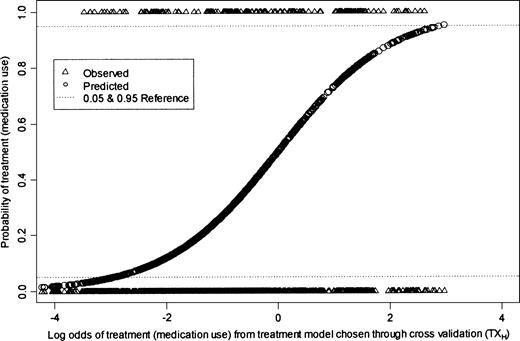
Graphical representation of evaluation of the experimental treatment assumption.
CONCLUSION
MSMs are an important advance for the analysis of complex epidemiologic data. Several methods, each with its own assumptions, are available for estimating causal parameters defined by MSMs. IPTW estimation has considerable appeal, because 1) it can be understood intuitively, even though the general concepts on which it relies (estimating functions) are more complex, and 2) existing routines (weighted least-squares regression) in popular software packages can be used. We have used an example for which the approximate “truth” of the effect of the treatment is known and was estimated within comparable data. We demonstrated the effect of misspecification of the treatment models on the effect estimate and evaluated the validity of the estimates with data on the same children. This example has provided an opportunity to implement IPTW under conditions where the ETA assumption was almost completely met.
Like other statistical applications, valid IPTW estimation relies on certain assumptions. Estimation methods for MSMs assume that there are no unmeasured confounders, just as do traditional conditional regression analyses. Theoretical insights demonstrate that the ETA assumption is a sine qua non for valid IPTW estimation (12). Practical violation of the ETA assumption requires the use of either G-estimation or the double-robust estimator. We have presented a relatively simple method of evaluating this assumption with empirical data and a graphic summary for assessing the results. We have demonstrated elsewhere the magnitude of the bias that can be introduced when this assumption is not met (12).
Software such as SAS can be used to implement IPTW; however, model-fitting and cross-validation require multiple steps, extensive programming, and substantial computing power. Our example shows that presentation of findings based on IPTW estimation with a single treatment model is inadequate. The selection of a treatment model based solely on AIC criteria led to biased estimation of the causal effect. The sensitivity of the estimates to the truncation of the treatment weights should be evaluated, and investigators who use IPTW estimation should be expected to undertake some level of formal model-fitting to justify the choice of the final weights used.
The Fresno Asthmatic Children's Environment Study was funded by the California Air Resources Board (contract 99-32).
Conflict of interest: none declared.
References
Bodnar LM, Davidian M, Siega-Riz AM, et al. Marginal structural models for analyzing causal effects of time-dependent treatments: an application in perinatal epidemiology.
Cole SR, Hernán MA, Robins JM, et al. Effect of highly active antiretroviral therapy on time to acquired immunodeficiency syndrome or death using marginal structural models.
Cook NR, Cole SR, Hennekens CH. Use of a marginal structural model to determine the effect of aspirin on cardiovascular mortality in the Physicians'
van der Laan MJ, Robins JM. Unified methods for censored longitudinal data and causality. New York, NY: Springer-Verlag,
Neugebauer R, van der Laan M. Why prefer double robust estimators in causal inference?
Robins JM, Hernán MA, Brumback B. Marginal structural models and causal inference in epidemiology.
van der Laan MJ, Dudoit S. Unified cross-validation methodology for selection among estimators and a general cross-validated adaptive epsilon-net estimator: finite sample oracle inequalities and examples. (U. C. Berkeley Division of Biostatistics Working Paper Series, paper 130). Berkeley, CA: Division of Biostatistics, University of California, Berkeley,
Tager IB, Haight T, Sternfeld B, et al. Effects of physical activity and body composition on functional limitation in the elderly.
Neugebauer R, van der Laan M. Locally efficient estimation of nonparametric causal effects on mean outcomes in longitudinal studies. (U. C. Berkeley Division of Biostatistics Working Paper Series, paper 134). Berkeley, CA: Division of Biostatistics, University of California, Berkeley,
Haight T, Neugebauer R, Tager I, et al. Comparison of the inverse probability of treatment weighted (IPTW) estimator with a naïve estimator in the analysis of longitudinal data with time-dependent confounding: a simulation study. (U. C. Berkeley Division of Biostatistics Working Paper Series, paper 140). Berkeley, CA: Division of Biostatistics, University of California, Berkeley,

